The simple quadratic spline discussed my previous post seems to be sufficient for interpolating particle positions between two GADGET-2 snapshots for the purposes of making animations, but it’s also possible to use a cubic spline for the task. The advantages of using a cubic spline are (1) it can be more accurate—especially in cases where the acceleration changes sign once between snapshots, and (2) the derivatives at the end-points of the spline match the derivatives specified in the input data. In the case of the quadratic spline, if the acceleration (second derivative) changes sign even once during the interval, the interpolation is poor and the derivative of the spline at the end points is not guaranteed to match the specified value. Thus, in the case of the quadratic spline, the derivative is generally discontinuous when moving from one interval to another. This doesn’t matter too much when making animations with reasonably small intervals, but it would be important for certain other situations. The disadvantage of the cubic spline is that it adds complexity.
Cubic spline interpolation seems to be quite popular. Derivations of the general method can be found in most textbooks on numerical methods. I’ll just discuss the specific result that’s useful for my application—the cubic spline in terms of the end-point positions and velocities. To derive the result, we just have to slightly modify the derivation given in the previous post. We add a jerk term \(\mathbf{j}(t)\) (third derivative of the position with respect to time) to the third and fourth Taylor expansions,
\[\mathbf{r}_{0}\approx\mathbf{r}(t)+(t_{0}-t)\mathbf{v}(t)+\frac{1}{2}(t_{0}-t)^2\mathbf{a}(t)\]
\[\mathbf{r}_{1}\approx\mathbf{r}(t)+(t_{1}-t)\mathbf{v}(t)+\frac{1}{2}(t_{1}-t)^2\mathbf{a}(t)\]
\[\mathbf{v}_{0}\approx\mathbf{v}(t)+(t_{0}-t)\mathbf{a}(t)+\frac{1}{2}(t_{1}-t)^2\mathbf{j}(t)\]
\[\mathbf{v}_{1}\approx\mathbf{v}(t)+(t_{1}-t)\mathbf{a}(t)+\frac{1}{2}(t_{1}-t)^2\mathbf{j}(t)\]
and solve the system of equations for \(\mathbf{r}(t)\). There are, of course, several ways of doing this. I’ll skip the details and show the end result. I defined \[\delta t \equiv t_1-t_0,\qquad \tau_0 \equiv t_0-t,\qquad \tau_1 \equiv t_1-t\]
In terms of these definitions,
\[\mathbf{r}(t)=\frac{\mathbf{r}_0\tau_1^2+\mathbf{r}_1\tau_0 ^2+\tau_0\tau_1(\mathbf{v}_1\tau_0 ^2-\mathbf{v}_0\tau_1^2)/\delta t}{\tau_1^2+\tau_0^2}\]
This can be written more compactly as
\[\mathbf{r}(t)=\frac{\mathbf{r}_0+\rho \mathbf{r}_1+(\rho \mathbf{v}_1-\mathbf{v}_0)\tau_1\tau_0/\delta t}{\rho+1}\]
where
\[\rho\equiv\frac{\tau_0^2}{\tau_1^2}=\frac{(t_0-t)^2}{(t_1-t)^2}\]
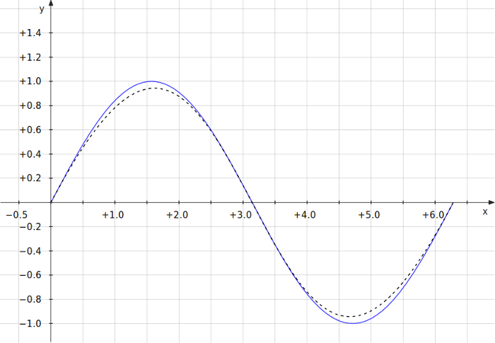
As an example, the cubic function generated by this technique when given values corresponding to \(\sin(x)\) at \(x=0\) and \(x=2\pi\) is
\[s(x)=\frac{(2\pi-x)(\pi-x)x}{x^2-2\pi x+2\pi^2}\]
In the plot below, \(\sin(x)\) is the blue curve and \(s(x)\) is the dotted black curve.